The Standard Model and the Higgs Boson
The Standard Model (SM) of particle physics is a remarkably successful and tested theoretical framework that describes the fundamental constituents of matter and their interactions. It classifies all known elementary particles into two broad categories: spin-1/2 fermions (quarks and leptons), which form the building blocks of matter, and spin-1 gauge bosons (photons, gluons, and the \(W^\pm\) and \(Z\) bosons), which mediate the electromagnetic, strong, and weak fundamental forces, respectively.

Where does the Higgs boson stand here?
One of the crucial requirements of the SM is a mechanism to generate the masses of these fundamental particles without violating the underlying mathematical symmetries of the theory. This is achieved through a scalar field. The fundamental fermions and the massive weak force carriers (\(W^\pm\) and \(Z\) bosons) acquire their intrinsic masses by continuously interacting with this field. A direct observable consequence of this field is the existence of a single, spin-0 scalar particle: Higgs boson (\(H\)).
In 2012, the ATLAS and the CMS collaborations at the LHC announced the historic discovery of a new scalar resonance with a mass of \(m_H \approx \text{125 GeV}\).
Subsequent experimental measurements have confirmed that the particle's properties strongly align with the predictions for the SM Higgs boson. With its mass now fixed, all other properties of the \(H\) boson are constrained by the SM.
Higgs Boson Production at the LHC
At the LHC, protons collide at ultra-high energies, specifically at a center-of-mass energy of \(\sqrt{s} = \text{13 TeV}\) for the 2016 data-taking period used in this analysis. At such high energies, the collision occurs at the quark level, and because of the large amount of energy available, many heavy particles (\(W^\pm,\ Z,\ H\)) are produced.
There are four primary production mechanisms for the SM Higgs boson at the LHC:
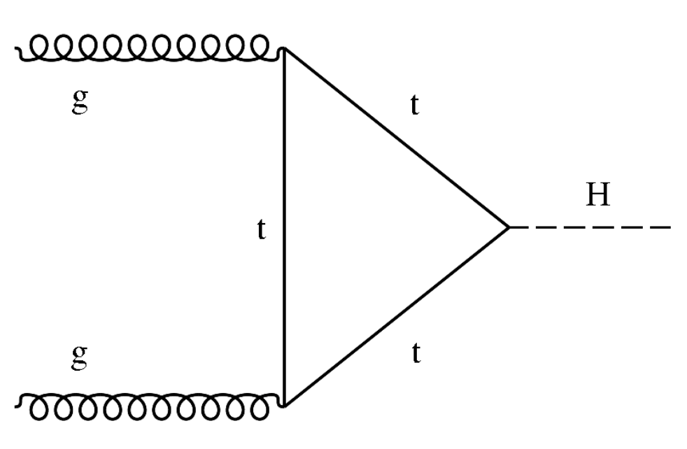
- Gluon-Gluon Fusion (ggH or ggF): Two gluons from the interacting protons fuse to produce a Higgs boson. Because gluons are massless, they cannot couple directly to the Higgs boson. This process occurs via a virtual loop of heavy quarks. The top quark, having the largest Yukawa coupling, dominates this loop exchange.
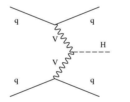
- Vector Boson Fusion (VBF): Two quarks from the incoming protons emit a gauge boson (\(W\) or \(Z\)), which then scatter and fuse to form a Higgs boson. This mode is characterized by two highly energetic forward jets in the detector.
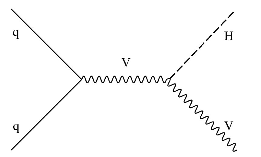
- Associated Production (VH): A quark and an antiquark annihilate to form an off-shell \(W\) or \(Z\) boson, which then radiates an \(H\).
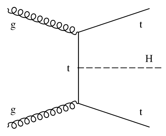
- Top Quark Associated Production (ttH): Two gluons or quarks fuse to produce a top-antitop quark pair along with an \(H\).
Dominance of Gluon-Gluon Fusion
This analysis specifically focuses on the ggH production mode. The choice to isolate this channel over others is driven by two primary kinematic and experimental factors:
- Cross-section Dominance: At a center-of-mass energy of \(\sqrt{s}\ =\ \text{13 TeV}\), ggH is by far the most abundant production mechanism. According to Handbook of LHC Higgs cross sections, the inclusive cross-section for ggH at 13 TeV is \(\sigma_{ggH}\approx \text{48.58 pb}\). This accounts for approximately 87% of the total Higgs boson production at the LHC. This overwhelming abundance ensures the maximum possible signal yield, providing a strong statistical foundation for the analysis.
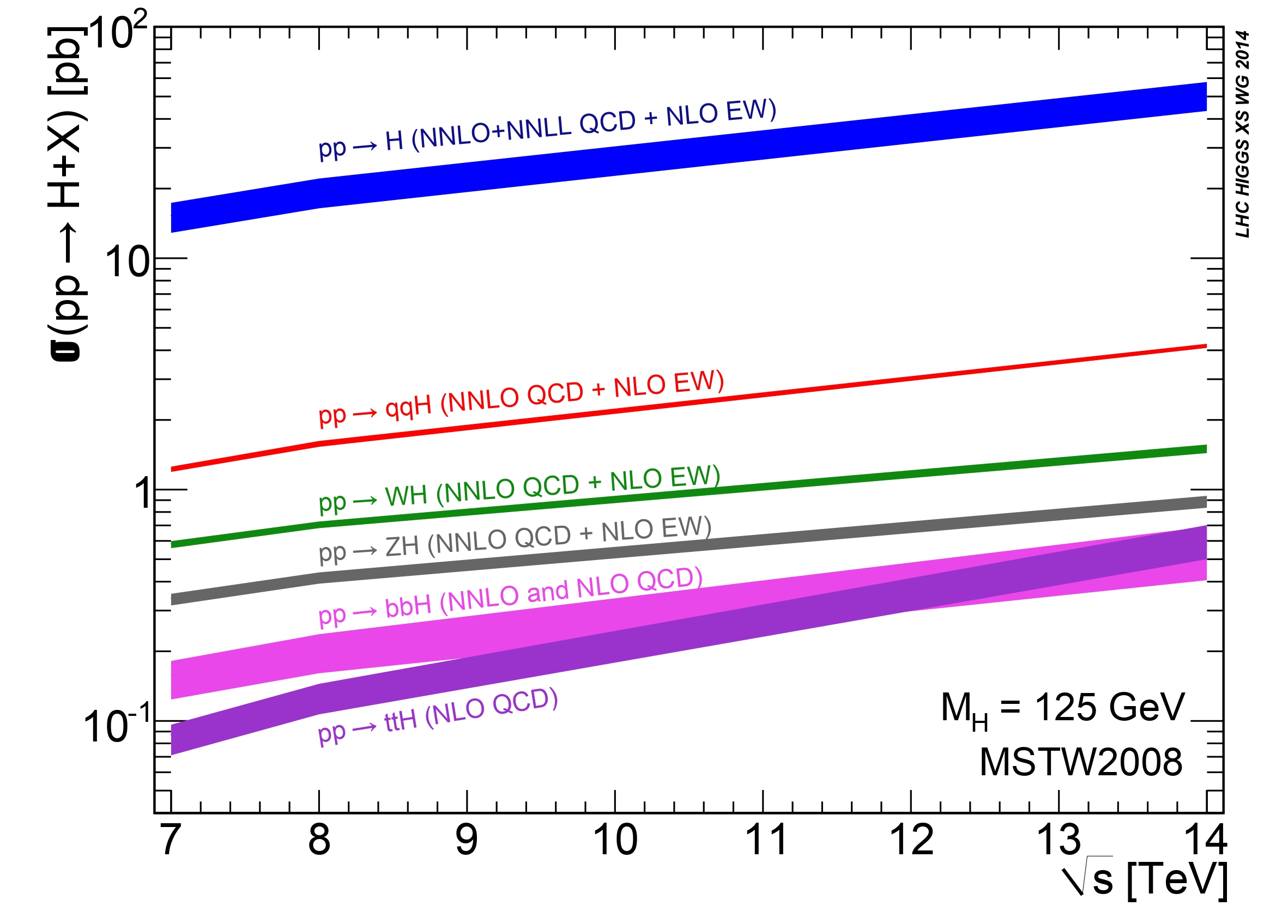
- Signal Cleanliness: Compared to other production modes, the ggH process offers a comparatively clean experimental topology. For example, the VBF channel, despite having the second-largest cross-section, is characterized by the presence of two highly energetic "forward" jets. Identifying these jets and removing them from the background requires complex jet selections, making the analysis highly sensitive to pileup in the detector region. Similarly, VH and ttH introduce additional heavy bosons or top quarks, making the final state cluttered with extra leptons and \(b\)-quarks. Thus, focusing on ggH allows for a cleaner extraction of the Higgs signal.
Higgs Boson Decay
Once produced, the Higgs boson is highly unstable and decays almost instantaneously. In the SM, the strength of its coupling to other fermions and bosons is proportional to their masses, meaning it preferentially decays into the heaviest kinematically available particle pairs.
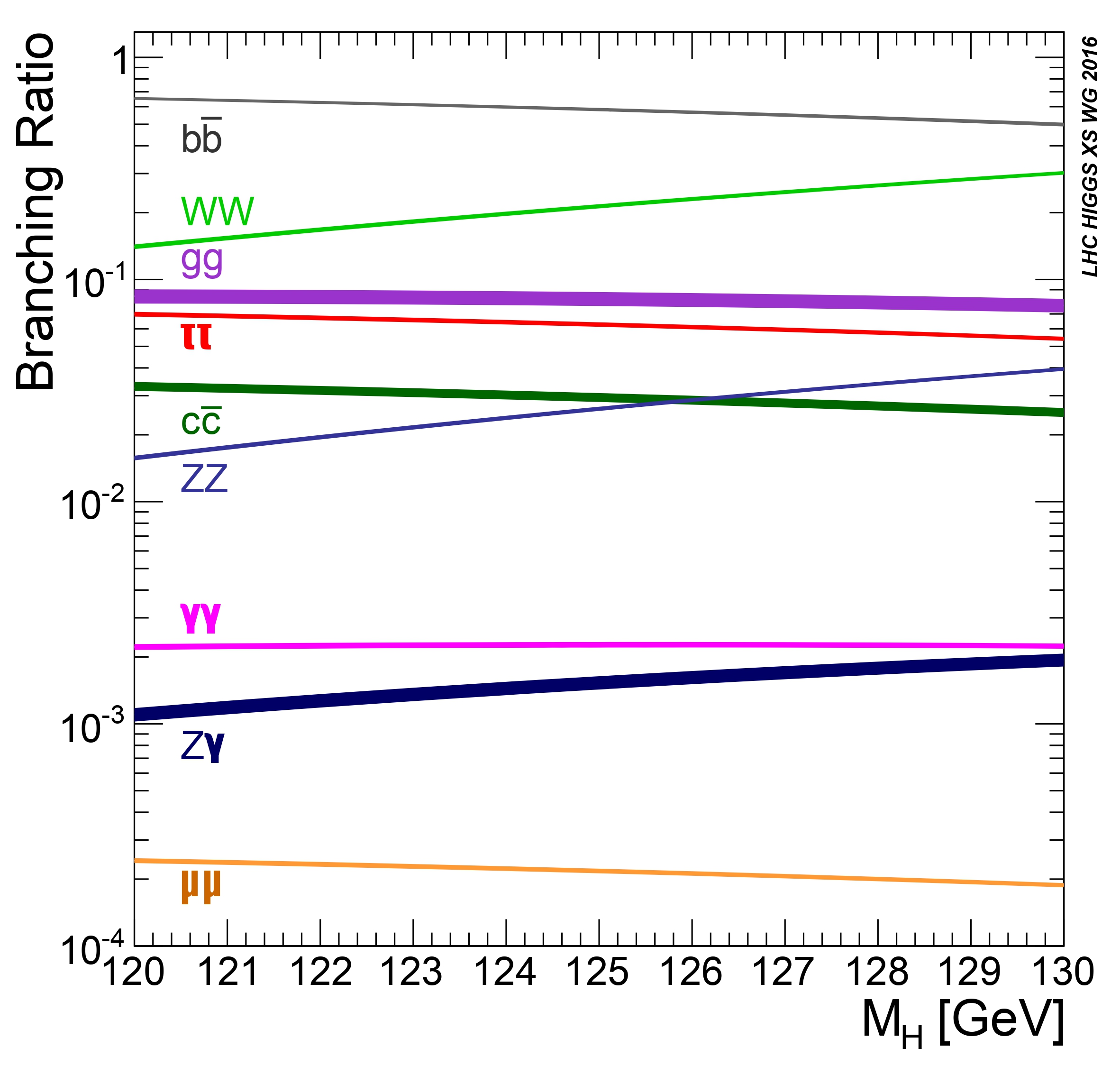
Using the precision calculations compiled in the Handbook of LHC Higgs cross sections: 4, for a Higgs boson with a mass of \(m_H\approx\text{125 GeV}\), the branching ratios are distributed as follows:
| Decay Channel | Branching Ratio (BR) |
|---|---|
| \(H \rightarrow b\bar{b}\) | 58.09% |
| \(H \rightarrow WW^{*}\) | 21.52% |
| \(H \rightarrow gg\) | 8.18% |
| \(H \rightarrow \tau^{+}\tau^{-}\) | 6.26% |
| \(H \rightarrow c\bar{c}\) | 2.88% |
| \(H \rightarrow ZZ^{*}\) | 2.64% |
| \(H \rightarrow \gamma\gamma\) | 0.227% |
| \(H \rightarrow Z\gamma\) | 0.154% |
| \(H \rightarrow \mu^{+}\mu^{-}\) | 0.022% |
Off-shell Production
Because the mass of the Higgs boson is less than twice the mass of an on-shell W or Z boson, one of the emitted vector bosons in these decay modes must be produced virtually, or off-shell, denoted by the asterisk.
Why the H to WW Channel Is Preferred
While the decay into a bottom-antibottom quark pair (\(H\to b\bar{b}\)) has the highest branching ratio, searching for it in a detector presents several challenges. The LHC produces an overwhelmingly vast background of strong-interaction processes (QCD multijet events) that perfectly mimic the hadronic final state, making precision measurements exceptionally difficult.
To bypass the massive hadronic backgrounds, this analysis focuses on the \(H\to WW^*\) decay mode. This channel offers many advantages for experimental physics:
-
High Event Yield: With the second-largest branching ratio (\(\approx \text{21.52}\%\)), it provides a substantial statistical sample compared to rarer decays.
-
Clean Signature: The leptonic decay of the \(W\) bosons (\(W \to \ell \nu\)) produces high-energy, isolated leptons that cleanly stand out from the overwhelming QCD backgrounds.
-
Drell-Yan Suppression: By strictly requiring the different-flavor final state (\(H \to WW^*\to e^{\pm}\mu^{\pm}\nu\bar{\nu}\)), the analysis easily bypasses the massive Drell-Yan background (\(Z/\gamma^* \to e^\pm/\mu^\pm\)) that plagues the same-flavor searches.
W Boson Decay Modes
To understand the final state topology of the event, we must examine the decay mechanisms of the intermediate vector bosons. A \(W\) boson decays in two primary ways:
- hadronically into a quark-antiquark pair (\(W\to q\bar{q}\)), or
- leptonically into a charged lepton and its corresponding neutrino (\(W \to \ell\nu\)).
While the hadronic decay is favored with a branching ratio of approximately 67.4%, it suffers from overwhelming QCD multi-jet backgrounds at the LHC. Conversely, the leptonic decay provides a much cleaner experimental signature. According to the baseline values established in the Handbook of LHC Higgs cross sections, the leptonic branching ratio for each specific flavor family (\(e,\ \mu,\ \tau\)) is mathematically symmetric at \(\approx\) 10.86%.
The Fully Leptonic Different-Flavor State
This analysis explicitly targets the fully leptonic final state, requiring both \(W\) bosons to decay into leptons. Furthermore, the selection is strictly narrowed to the different-flavor (\(e^\pm \mu^\pm\)) final state.
While incorporating same-flavor events (\(e^+e^-\) or \(\mu^+\mu^-\)) would normally increase the raw signal yield, they introduce a massive and difficult-to-handle background from Drell-Yan processes (\(Z/\gamma^* \to \ell^+\ell^-\)). Because Drell-Yan interactions almost always produce same-flavor lepton pairs, requiring exactly one electron and one muon suppresses this \(Z\)-boson resonance background, yielding a highly pure signal region.
The Expected Yield Calculation Chain
By synthesizing the production cross-section of the Higgs boson with the sequential branching ratios of its decay products, the expected theoretical yield for the exact signal process can be mathematically formalized.
For the \(gg\to H \to WW \to e^\pm\mu^\pm\nu\bar{\nu}\) channel, the theoretical cross-section (\(\sigma_{signal}\)) is calculated as:
\(\sigma_{signal} = \sigma(gg\to H) \times \text{BR}(H \to WW) \times \text{BR}(W \to e\nu) \times \text{BR}(W \to \mu\nu)\times 2\)
Charge-Flavor Permutations
The factor of 2 accounts for the two possible charge-flavor combinations of the final state: \(W^+ \to e^+\nu_e\), \(W^- \to \mu^-\bar{\nu}_\mu\) and \(W^+ \to \mu^+\nu_\mu\), \(W^- \to e^-\bar{\nu}_e\).
Experimental Signature in the Detector
Understanding how the process "looks like" in the detector is a crucial first step in our search.
The Visible: Electrons and Muons
The charged leptons produced in the \(W\) boson decays are the primary visible handles of the signal. They must be accurately reconstructed and identified by the various sub-detectors:
-
Electrons (\(e^\pm\)): An electron leaves a curved trajectory in the inner silicon tracker and subsequently deposits energy into the Electromagnetic Calorimeter (ECAL), producing an electromagnetic shower.
-
Muons (\(\mu^\pm\)): As minimum-ionizing particles, muons leave a track in the inner silicon tracker, pass through the ECAL and Hadronic Calorimeter (HCAL) with negligible energy loss, and are finally reconstructed by the dedicated muon chambers located in the outermost layers of the CMS detector.
The Invisible: Missing Transverse Energy (MET)
Being chargeless and almost massless, neutrinos pass through the entire detector volume without leaving a single trace.
Because the initial protons collide head-on along the beam axis (\(z\)-axis), the net momentum of the system in the transverse plane (\(x-y\) plane) is strictly zero. By using conservation of momentum, the presence of neutrinos is inferred by calculating the vector sum of the transverse momenta of all visible particles reconstructed in the event. Any imbalance in the sum is quantified as Missing Transverse Energy (\(E_T^{miss}\) or MET). In this analysis, large MET is expected because neutrinos are present in the final state.
Kinematic Variables and Signal Discrimination
In any analysis, the final state of the process can be represented by specific kinematic variables. In this analysis, we will use a few such key variables to represent our signal process and distinguish it from the background:
- Transverse Mass of Higgs (\(m_T^H\)): Because the two escaping neutrinos prevent the full reconstruction of the Higgs invariant mass, we rely on the transverse mass. Formulated using the transverse momentum of the dilepton system and the missing transverse energy, it forms a broad edge around the \(m_H \sim 125 \text{ GeV}\) rather than a sharp resonance peak.
- Transverse Momentum of the Dilepton System (\(p_T^{\ell\ell}\)): The combined transverse momentum of the visible electron and muon.
- Dilepton Invariant Mass (\(m_{\ell\ell}\)): The invariant mass calculated directly from the four-momenta of the visible electron–muon pair.
- Angular Separation (\(\Delta\phi_{\ell\ell}\)): The absolute difference in the azimuthal angle between the electron and muon in the transverse plane. It gives the separation between the two leptons in the transverse plane.